Finding the likely causes when potential explanatory factors look alike
Suppose you are a scientist interested in investigating if there is a link between exposure to car pollutants during pregnancy and the amount of brain white matter at birth. A starting hypothesis you would like to test could be: is an increase of a specific pollutant associated with a reduction (or increase) of white matter in newborns? A typical study to test this hypothesis would involve recruiting pregnant women, measuring the average amount of pollutants they are exposed to throughout their pregnancy, and measuring the newborn’s proportion of white matter, which is a measure of connectivity. After the collection, the data analysis would involve assessing if at least one of the car pollutants is correlated with the newborn’s brain measurements. It is now well established that exposure to car pollutants during pregnancy is associated with reduced white matter proportion in newborns. A natural follow-up question would be among all these car pollutants which is likely to cause a reduction in white matter? That is when things become more tricky.
Because cars tend to produce the same amount of each pollutant (or at least the proportion of pollutants they emit is somewhat constant), we observe little variation in car pollutant proportion over time in a given city. It would be even worse if we only studied women from the same neighborhood and recruited them during a similar period of time (as we expect the car pollutants to be quite homogeneous within a small area). The main difficulty in trying to corner a potential cause among correlated potential causes is that if pollutant A ( e.g., Carbon Monoxide CO) affects the newborn white matter but pollutant B (e.g., Carbon Dioxide C2O) is often producing along with pollutant A, it is likely that both pollutants will be correlated with newborn white matter proportion.
Correlation has been a primary subject of interest since the early days of statistics. While correlation is often a quantity of inferential interest (e.g., predicting house price given its surface), in some cases, it can plague an analysis as it is hard to distinguish between potential causes that are correlated (as described above).
Assume now that exactly two pollutants among four that are affecting newborn white matter. Pollutants 1 and 3, say — and that these two pollutants are each completely correlated with another non-effect pollutant, say pollutants 1 and 2 are perfectly correlated and pollutants 2 and 4. Here, because the pollutants are completely correlated with a non-effect pollutant, it is impossible to confidently select the correct pollutants that are causing health problems. However, it should be possible to conclude that there are (at least) two pollutants that affect white matter, for the first pollutant that affects white matter it is whether (pollutant 1 or pollutant 2), for the first pollutant that affects white matter it is whether (pollutant 3 or pollutant 4).
This kind of statement (pollutant 3 or pollutant 4) is called credible sets in the statistical genetic literature. Credible sets are generally defined as follows. A credible set is a subset of the variables that have at least 95% to contain at least one causal variable. In our example, the pollutants are the variables. Inferring credible sets is referred to as fine mapping.
Until recently, most of the statistical approaches were working well for computing credible sets in the case that exactly one pollutant affects newborn white matter. Recent efforts led by the Stephens’ lab and other groups suggest enhancing previous models by simply iterating them through the data multiple times. For example, suppose I have made an initial guess for the credible sets for the first effect pollutant. Now, I can remove the effect of the pollutant from my data and guess the credible sets for the second effect. Once this is done, we can refine our guess for the first pollutant by removing the effect of the second credible set from the data and continuing to repeat this procedure until convergence.
The example we presented above is quite simple as a maximum of a hundred pollutants and derivatives are being studied, and they can be potentially tested one by one in a lab using mice. The problem becomes much harder in genetics, where scientists try to understand the role of hundreds of thousands of variants on molecular regulation. And in fact, genetic variants tend to be much more correlated than car pollutants. And this complexity increases as we try to understand more complex traits. For example, instead of just trying to see if exposure to car pollutants affects the white matter at birth, we could see if that affects the proportion of white matter throughout childhood.
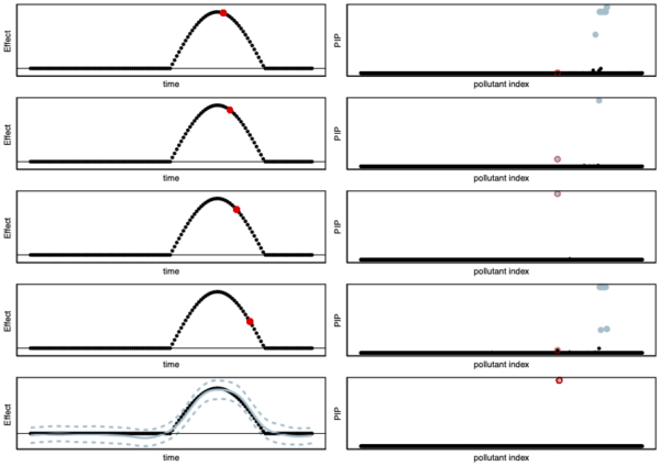
Our current work is generalizing the iterative procedure described here to a more complex model. One of the main difficulties is to find a good trade-off between model complexity and computational efficiency. More complex models capture more subtle variation in the data but are more costly to estimate. We use ideas from signal processing methods (wavelet) to perform fast iterative procedures to corner genetic variants (or car pollutants) that affect dynamic or spatially structured traits (e.g., white matter development throughout childhood or DNA methylation). We present some of the advantages of our new work in Figure 1.
Coming back to our earlier example where pollutants 1 and 3 affect white matter. The main problem with fine-mapping pollutants that affect temporally-structured traits is that standard fine-mapping may suggest that pollutant 1 affects white matter proportion at birth but then may suggest that pollutant 2 affects white matter at three months. Thus leading to inconsistent results throughout childhood. Using a more advanced model that can look at each child’s trajectory (instead of at each time point separately as normally done) allows for more consistent and interpretable results. We illustrate this advantage in Figure 1.
This work was funded by the Eric and Wendy Schmidt AI in Science Postdoctoral Fellowship, a Program of Schmidt Futures.

Towards New Physics at Future Colliders: Machine Learning Optimized Detector and Accelerator Design
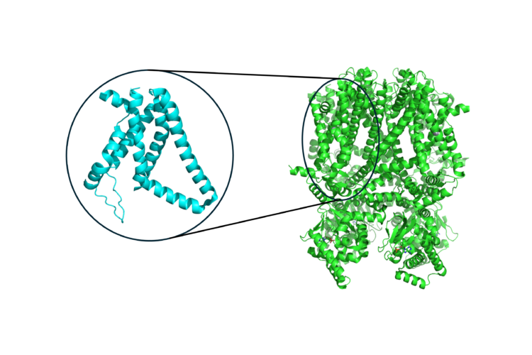
Uncovering Patterns in Structure for Voltage Sensing Membrane Proteins with Machine Learning
An Intro to Gravitational-Wave Astronomy